
Random Forest with H2O
Random forests are a one of my favorite machine machine learning methods. I’ve found them to be incredibly powerful in predicting a number of items in my work, but often run into performance issues running them on my local machine. A coworker recommended the R package H2O – an open source, high performance, in-memory machine learning platform. It has been a game changer in terms of my being able to run efficient predictive models locally. In this post, I will walk though implemenation of a random forest using a long passed Kaggle competition, Don’t Get Kicked.
I chose this dataset since it has both numeric and categorical predictors, a mix I often find in my workspace. The goal of this Kaggle competition is essentially to predict which cars will be “lemons” when bought at auction. Download the training data to get started. There is also an accompanying data dictionary if you are interested in knowing the variable definitions.
One last note before digging into the reading. Markdown has trouble working with the H2O environment. So, I ran the code in a separate workbook and have pasted in the code output/images separately into my document. I also did not set a seed, so your results (if you choose to run this) may be slightly different from my own.
Data Setup
First, I will read the data and clean it up a bit.
# read the data
carvana <- read.csv(paste(your_file_path, "training.csv", sep = ""))

# remove some columns that I don't like
carvana$RefId <- NULL
carvana$PurchDate <- NULL
carvana$WheelTypeID <- NULL

# the data needs some cleaning & structuring
# there are some "NULL"s and blanks that I will convert to NA
carvana <- data.frame(lapply(carvana, as.character), stringsAsFactors = FALSE)
carvana[carvana == ""] <- NA
carvana[carvana == "NULL"] <- NA

# converting to factor variables
varFactor <- c("IsBadBuy", "Auction", "Make", "Model", "Trim", "SubModel", "Color", "Transmission",
               "WheelType", "Nationality", "Size", "TopThreeAmericanName", "PRIMEUNIT", "AUCGUART", "BYRNO",
               "VNZIP1", "VNST", "IsOnlineSale")
carvana[varFactor] <- lapply(carvana[varFactor], as.factor)

# converting to numeric variables
# note: "VehYear" could also used as a factor
varNumeric <- c("VehYear", "VehicleAge", "VehOdo", "MMRAcquisitionAuctionAveragePrice", "MMRAcquisitionAuctionCleanPrice",
                "MMRAcquisitionRetailAveragePrice", "MMRAcquisitonRetailCleanPrice", "MMRCurrentAuctionAveragePrice",
                "MMRCurrentAuctionCleanPrice", "MMRCurrentRetailAveragePrice", "MMRCurrentRetailCleanPrice",
                "VehBCost", "WarrantyCost")
carvana[varNumeric] <- lapply(carvana[varNumeric], as.numeric)
H2O and Random Forest
Now that the data has been formatted, let’s run the random forest model. Since I will be using H2O, I will need to initialize a local cluster before running the model. I will also be using a 75% of the data as a training set and 25% as the testing set. There is a separate testing data set available on Kaggle. If you wish to use the entire training.csv file as training set and the test.csv file as the test set, you could certainly do that too.
# load the pacakge
library(h2o)

# disable the progress bar (this just annoys me)
h2o.no_progress()

# initialize local cluster
localH2O <- h2o.init(nthreads = -1)

# convert dataset to h2o object
carvana_h2o <- as.h2o(carvana)

# create training and testing sets
carvana_h2o <- h2o.splitFrame(carvana_h2o, ratios = 0.75, destination_frames = c("train", "test"))
names(carvana_h2o) <- c("train", "test")

# creating a list of features for the model
inputModel <- names(carvana[-1])

# building the random forest model
rfCarvana <- h2o.randomForest(training_frame = carvana_h2o$train, validation_frame = carvana_h2o$test, x = inputModel, y = "IsBadBuy", ntrees = 100, stopping_rounds = 2)
In this example, I just threw all the variables into the model. I would typically do a separate analysis to determine which features to include in the model, but let’s skip over that for now. Next, we will take a look at variable importance and some metrics from the validation set.
Validation Metrics
Let’s see how our model performed. The output below summarizes the model performance on the test set of data used (the 25% held out from the training.csv).
# print metrics from the validation set
rfCarvana@model$validation_metric
## H2OBinomialMetrics: drf
## ** Reported on validation data. **
## MSE: 0.08770201
## RMSE: 0.2961452
## LogLoss: 0.3104513
## Mean Per-Class Error: 0.3566561
## AUC: 0.7447409
## Gini: 0.4894817
##
## Confusion Matrix for F1-optimal threshold:
## 0 1 Error Rate
## 0 15237 697 0.043743 =697/15934
## 1 1461 721 0.669569 =1461/2182
## Totals 16698 1418 0.119121 =2158/18116
##
## Maximum Metrics: Maximum metrics at their respective thresholds
## metric threshold value idx
## 1 max f1 0.296480 0.400556 144
## 2 max f2 0.103983 0.479038 280
## 3 max f0point5 0.544554 0.537988 71
## 4 max accuracy 0.544554 0.900309 71
## 5 max precision 0.857207 1.000000 0
## 6 max recall 0.005868 1.000000 395
## 7 max specificity 0.857207 1.000000 0
## 8 max absolute_mcc 0.544554 0.397583 71
## 9 max min_per_class_accuracy 0.110008 0.670516 274
## 10 max mean_per_class_accuracy 0.151616 0.676490 236
##
## Gains/Lift Table: Extract with `h2o.gainsLift(<model>, <data>)` or `h2o.gainsLift(<model>, valid=<T/F>, xval=<T/F>)`Whenever I run a random forest model, I always look at the variable importance output. It is interesting to see which variable perform well and which do not. Accroding to the H2O documentation …
“Variable importance is determined by calculating the relative influence of each variable: whether that variable was selected during splitting in the tree building process and how much the squared error (over all trees) improved as a result.”
In our case, “WheelType” (The vehicle wheel type description (Alloy, Covers, Special)) was the stongest performer.
# variable importance
h2o.varimp(rfCarvana)
## Variable Importances:
## variable relative_importance scaled_importance percentage
## 1 WheelType 53910.425781 1.000000 0.183251
## 2 SubModel 35982.921875 0.667458 0.122312
## 3 VNZIP1 33045.710938 0.612974 0.112328
## 4 BYRNO 25883.117188 0.480113 0.087981
## 5 Color 16262.140625 0.301651 0.055278
##
## ---
## variable relative_importance scaled_importance percentage
## 25 TopThreeAmericanName 1692.602905 0.031397 0.005753
## 26 AUCGUART 654.976257 0.012149 0.002226
## 27 Nationality 643.357788 0.011934 0.002187
## 28 Transmission 620.358093 0.011507 0.002109
## 29 PRIMEUNIT 540.431274 0.010025 0.001837
## 30 IsOnlineSale 235.844467 0.004375 0.000802The variable importance plot displays the scaled importance.
# plot of variable importance
h2o.varimp_plot(rfCarvana)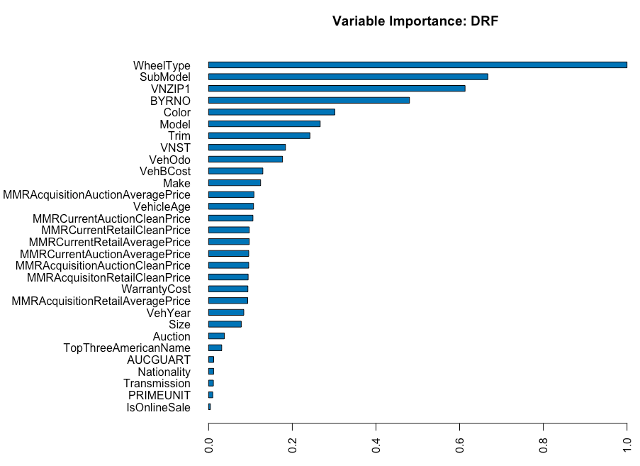
Lastly, I will take a look at the ROC curve. Our model is better than making random predictions - yay!
# build and plot the ROC curve
rfROC <- h2o.performance(rfCarvana, newdata = carvana_h2o$test)
plot(rfROC)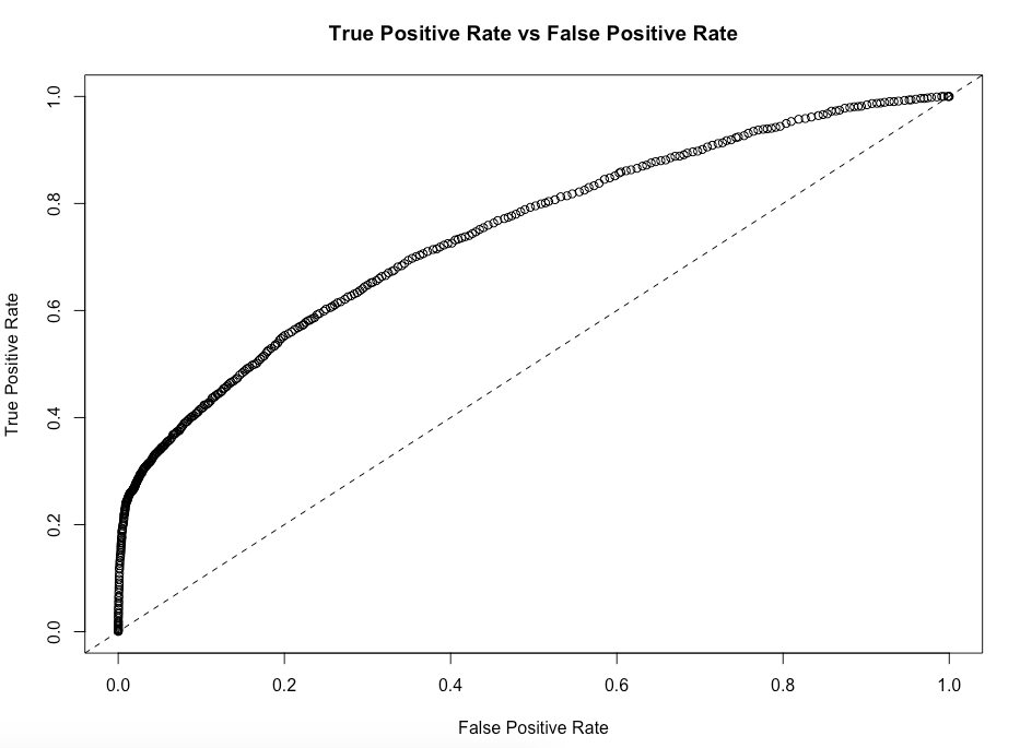
Cluster Shut Down
If you are satisfied with the result, go ahead and shutdown the cluster you have running locally. However, if you would like to go back and refine the model you built, shut it down later.
# shut down the local cluster
# if you want to refine your model futher, do not run this line
h2o.shutdown(prompt = FALSE)
Submission to Kaggle
If you want to submit this random forest model (or some other tweaked model from my code above) to Kaggle, the code I used to create the submission file is below. In order for your submission to be accepted, you must make predictions on the test.csv dataset provided on Kaggle website. You will have to import and do the data preprocessing above in order to get a result they will accept (hey … it will be good practice!).
This solution will get you about middle of the pack on Kaggle.
# get predicions for test set
# note: the test dataset I called "carvana_test" and performed the preprocessing above
preds <- h2o.predict(rfCarvana, carvana_test)
preds <- as.data.frame(preds)

# create the submission dataframe
submission <- cbind(refID, preds$predict)
names(submission) <- c("refID", "IsBadBuy")

# write the file to csv
write.csv(submission, file = paste(your_file_path, "submission.csv", sep = ""), row.names = FALSE)